Average Rate of Change, Math Help and Tutoring

Need one-on-one tutoring with me? I teach all of this material! Contact me for a quick response on your needs.
Want my FULL version of these notes with more worked examples and help? Click here.

Introduction

We begin this chapter by discussing an important concept in algebra-level math which will ultimately lead to the fundamentals of calculus. Many times, in real-world applications, we want to find the rate at which something is changing (increasing or decreasing). This “something” could be anything from the cost of conducting business, to the value of a stock, to the water level in a body of water. Being able to calculate the rate at which a quantity is changing is valuable in making predictions about where its actual level will be after some time, or where it may have been in the past before being measured.

We will start out in this section by finding what’s called the average rate of change for a curved function between two points in order to understand how the function is evolving in a very surface-level way. We will then expand on this process, using limits, to find the instantaneous rate of change right at a specific point, which has many applications with functions of many varieties, and ultimately leads to the calculus construct called the derivative.

The Rate of Change Defined

As described above, the rate of change is how quickly something is increasing or decreasing over time (or more generally, over the value of the independent variable, which need not be time):

The rate of change of a function is how quickly the dependent variable evolves over changes in the independent variable.

For a linear function, this is really straightforward! The rate at which the dependent variable evolves with respect to the independent variable in a linear relationship is the same throughout the line, and is represented by the slope of that line:

The rate of change for a linear function is simply its slope.

You’ll find a much, much more detailed description, with associated examples and graphics on this principle, in my full notes on this section.

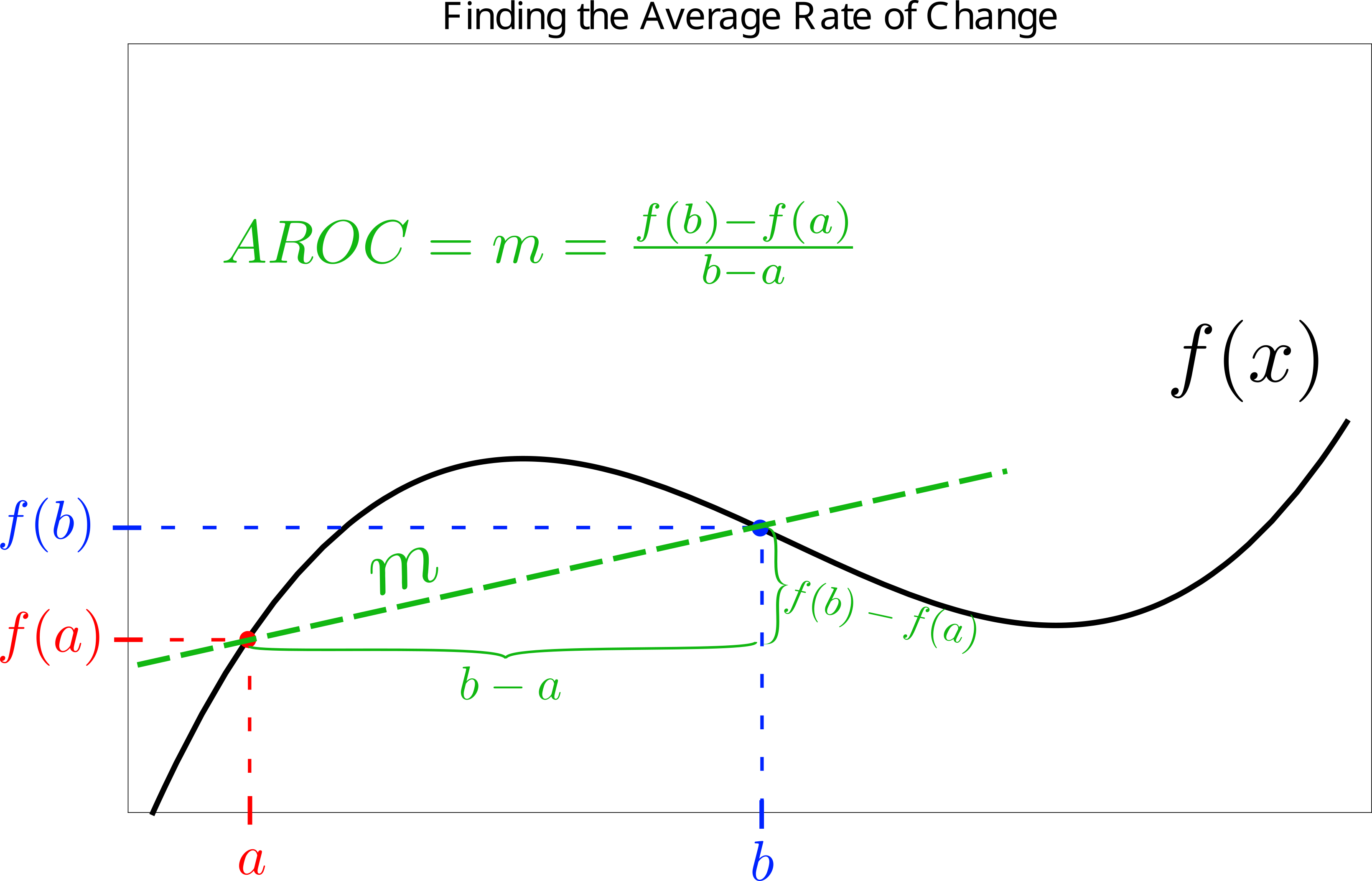
The Average Rate of Change

What about finding the rate of change for a curved function? Well, this is more complicated because the rate of change itself keeps changing, which means we must either find how quickly it’s changing right at a moment, or else talk about how much it changed on average to get us to this point. The latter is called the average rate of change, and it can be calculated for a function with all sorts of curvature according to the following formula:

The average rate of change for a function $f(x)$ from $x = a$ to $x = b$ is

(1) $\begin{equation*} AROC = \frac{f(b) - f(a)}{b - a} \end{equation*}$

The line that moves through the two points of consideration, of which the $AROC$ in Equation 1 is the slope, has a specific name.

A line that connects two points with finite separation on a function is called a secant line.

Here is a visual representation of this situation, which shows why the slope of the secant line through the two points of interest is as described above:

Why is this an Average?

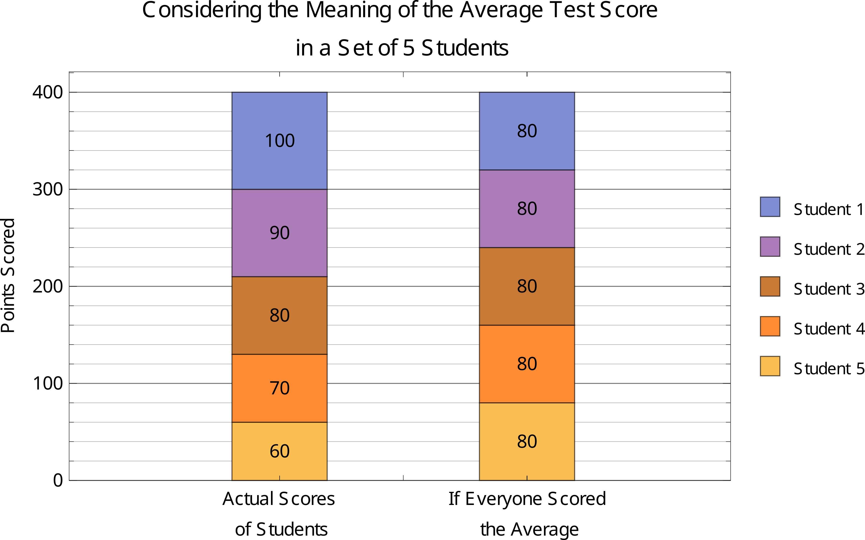
Although I go into much more detail about the important concepts in this section in my full notes, I’ll reproduce a key analogy used in those notes here for explanation. When a quantity is “averaged”, we find the value such that, if the quantity had been exclusively equal to this value, the global picture would have been the same over the interval of consideration. For example, if the scores that 5 different students received on a test were 60, 70, 80, 90, and 100, respectively, we say that the “average” score (the mean, here) was 80, because an equal amount of points was scored on each side of this average (30 total points below and 30 total points above). That is, the total points scored would have been the same if everyone had scored this average number (400 total points either way). This is the important point. You can see a visual breakdown of this principle below; the total points scored would have been the same if everyone scored the average score of 80.

Much like how the average test score is the value that would produce the same total score among all the students if they had all scored that value instead, the average rate of change is the rate at which the function would have accumulated the same change if it had only increased at that constant rate throughout the entire interval of consideration. You’ll find much more detail on this here.

Basic Examples

Let’s look at some examples!

Example 1

Find the average rate of change of the function $y = -4x^2$ from the point $(1,-4)$ to the point $(2,-16).$

Finding the average rate of change for this function over this interval is as simple as using Equation 1. That proceeds as follows:

$AROC = \frac{y(b) - y(a)}{b-a} = \frac{-16 - (-4)}{2 - 1} = -12$

It’s also worth noting that, since the $x$ -coordinate $a$ is less than $b$ (to the left of it) in the $AROC$ formula, you should always choose the more rightward point as the one used for $(b, f(b))$ in the formula. Reversing the order will yield the same result of negative 12, however this doesn’t mean you’ve found the rate of change going “backwards” to the left; the rate of change formula exclusively calculates the rate while going “forward”.

Example 2

Find the average rate of change for $f(x) = 4x^2 - 6$ from $(1,-2)$ to $(3,30)$ .

Using the same equation, we get

$AROC = \frac{30 - (-2)}{3 - 1} = 16$

I give some graphical plots on many of the examples in my full notes to show how the average rate of change, secant line, and slope thereof, all relate.

Example 3

Find the average rate of change for $g(x) = -2x^3 - 4x^2 + 2$ from $x = -2$ to $x = 1$ .

Although we don’t know the respective $y$ -coordinates for these two points, we can find them by plugging the $x$ -values into $g(x)$ . Plugging in produces

$g(-2) = -2(-2)^3 - 4(-2)^2 + 2$

$= 2$

and

$g(1) = -2(1)^3 - 4(1)^2 + 2$

$= -4$

The $AROC$ formula produces

$AROC = \frac{-4 - 2}{1 - (-2)} = -2$

Example 4

Find the average rate of change for $y = \sqrt{x} + 1$ from $x = 0$ to $x = 16$ .

Finding that $y(0) = 1$ and $y(16) = 5$ , we get

$AROC = \frac{5 - 1}{16 - 0} = \frac{1}{4}$

Example 5

Find the $AROC$ for $y = 1/x$ from $x = 0.5$ to $x = 1$ .

Finding the respective $y$ -values and plugging in produces

$AROC = \frac{y(1) - y(0.5)}{1 - 0.5} = \frac{1 - 2}{0.5}$

$= -2$

Advanced Examples

Although you’ll find many more examples using the average rate of change (a common AP test topic!) in my full notes on this section, here are a few to get you started.

Example 6

The function $y = 1/x^2$ has an average rate of change of -1/2 from $(1,1)$ to what other coordinate, traversing rightward?

We can proceed with the normal $AROC$ formula with the unknowns $x = b$ and $y(b),$ while also noting that $y(1) = 1:$

$AROC = -\frac{1}{2} = \frac{y(b) - 1}{b - 1}}$

How do we proceed from here? Well, we know that $y(b) = \frac{1}{b^2}$ , so we can solve accordingly:

$-\frac{1}{2} = \frac{\frac{1}{b^2} - 1}{b - 1}$

We could cross-multiply and solve, but a better way is multiplying both sides by $-b^2$ , producing

$\frac{1}{2}b^2 = \frac{-1 + b^2}{b-1} = \frac{(b-1)(b+1)}{b-1} = b+1$

It’s important to know that the $(b - 1)$ term can only be divided away in the fraction assuming that $b \neq 1$ , or else we’d be dividing by zero. However, the $b = 1$ “solution” corresponds to the same $x$ -coordinate that we started at, which is clearly invalid, so it can be safely discarded. Continuing, we have

$\frac{1}{2}b^2 = b+1 \Rightarrow b^2-2b-2 = 0$

Using the quadratic equation here produces

$b = \frac{2 \pm \sqrt{4-4(1)(-2)}}{2} = 1 \pm \sqrt{3}$

Choosing the minus sign in this result produces a negative value of $b$ , which is not an $x$ -value to the right of $(1,1)$ . So, our solution is $b = 1+\sqrt{3}$ . The coordinate requires a $y$ -value, which is

$y(b) = \frac{1}{(1+\sqrt{3})^2} = \frac{1}{4+2\sqrt{3}} = 1 - \frac{\sqrt{3}}{2}$

when the conjugate multiplication is performed to remove the radical from the denominator.

We can always check our answer. Is the $AROC$ equal to $-\frac{1}{2}$ between these points? Pulling from above,

$AROC = \frac{(1-\frac{\sqrt{3}}{2}) - 1}{(1+\sqrt{3}) - 1} = \frac{-\frac{\sqrt{3}}{2}}{\sqrt{3}} = - \frac{1}{2}$

as desired! The other point is therefore $(1+\sqrt{3},1-\frac{\sqrt{3}}{2}).$

Example 7

Consider the following table, which records the profit a company made in millions of dollars, $P(t)$ , as a function of time in months. Over what 2-month interval did the company’s profits have the highest average rate of change? Note that profits are tallied at the end of a month, so a 2-month interval spans exactly 3 entries on the table.

$\begin{tabular}{ | c | c | c | c | c | c | c |}\hline$t$ (months) & 1 & 2 & 3 & 4 & 5 & 6 \\ \hline \hline$P(t)$ (\$M) & 0.00 & 0.45 & -0.23 & 1.54 & 1.12 & 1.49 \\ \hline\end{tabular}$

Notice that for all 2-month intervals (which are from month 1 to month 3, 2 to 4, 3 to 5, and 4 to 6), the denominator in the $AROC$ formula is always 2. Therefore, the interval with the largest $AROC$ must also have the largest numerator, which is the difference between the ending and starting profit values, or $P(b) - P(a)$ .

Calculating the differences in the profits for each of these intervals produces

$\begin{tabular}{ | c | c | c | c | c |}\hline Time Intervals & 1 \to 3 & 2 \to 4 & 3 \to 5 & 4 \to 6 \\ \hline \hline$P(b) - P(a)$ (\$M) & -0.23 & 1.09 & 1.35 & -0.05 \\ \hline\end{tabular}$

Therefore we see that the period from months 3 to 5 had the largest average rate of change in the profits for this company. On average, the company made $1.35 million per month during this period. Note that if the time intervals hadn’t been equally sized, you wouldn’t be able to disregard the denominator while using the $AROC$ formula.

Need more? Here you can get the full version of these notes!

Professional Math Tutoring Expertise

alex@mathhelpandtutoring.com

Average Rate of Change